Improved Group Average Dense Connectome for 500 Subjects R468

Type: Other

Correcting for the HCP rfMRI "Mound and Moat" ("Ring-of-Fire") Effect in Seed-based HCP Group Average Connectivity Data

Jesper Andersson, Matt Glasser, Christian Beckmann, David Van Essen, Steve Smith
April 2015

I. Summary of The M&M (RoF, or ripple) phenomenon

Seed-based connectivity analysis of the resting state HCP data (e.g., from previously released but subsequently withdrawn group-averaged dense connectome datasets) may show rings (or 'ripples') of lower (sometimes even negative) correlation encircling the seed voxel, as in the illustration below. This pattern looks counter-intuitive and neurobiologically implausible, and it therefore warrants explanation.

The analysis below provides evidence that multiple independent factors contribute to the observed ripple effect.

Spatially-dependent unstructured noise. Unstructured fMRI noise may have spatial dependencies, arising from the nature of the image acquisition, reconstruction and the interpolation methods used in motion/distortion correction and atlas registration.
Abrupt PCA truncation. Abrupt truncation of PCA components used for generation of a dense connectome can contribute to extensive rippling in regions of low SNR.

Of these, the second is the most significant for group average analysis from large numbers of subjects, including the recent HCP 500-subject release. The ripple effect from this cause can be essentially eliminated by applying an appropriate PCA-eigenvector weighting (rolloff) function, as described below. This rolloff strategy has the added benefit of improving SNR relative to the previously released dense connectome. The improved dense connectome (file name HCP_S500_R468_rfMRI_MIGP_d4500ROW_zcorr.dconn.nii) is now available via ConnectomeDB:

https://db.humanconnectome.org/data/projects/HCP_900

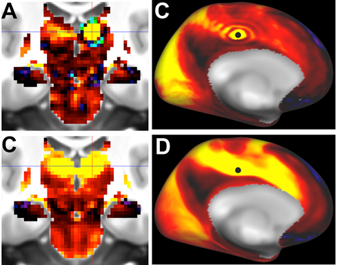
Fig.1. Top row: Ripple/Ring-of-Fire effects for a subcortical seed (panel A, thalamus) and a cortical seed (panel B, cingulate cortex) using abrupt truncation of 4500 PCA components. Bottom row. No ripple effect in either region after using a rolloff function for the PCA-eigenvector weighting (see text).

II. What do we estimate with seed based correlation?

When performing a seed-based analysis we extract a time-series from a 'grayordinate' (voxel or surface vertex) and then calculate the correlation between that and the time-series from every other grayordinate. When a region is positively correlated with the seed this provides evidence that it might be functionally connected to the seed.

However, the observed signal in a voxel (or surface vertex) includes a mixture of biologically relevant signal, structured noise (e.g., scanner and physiological artifacts) and 'unstructured' noise (e.g., MRI thermal white noise). We are only interested in correlations pertaining to the neuronal signal and go to great lengths to reduce the structured noise through pre-processing of the data. Pure 'white' noise, because it is (spatially) white, is not a problem except for reducing the 'SNR' of the final correlation map.

II.1. Unstructured MRI noise may not be perfectly 'white'

If noise is truly white, it should be independent across voxels. This means that if we take a large number of pairs of neighbouring voxels, calculate the correlation between the voxels in each pair, and average those correlations, the mean should be zero. With a relatively simple neuroimaging protocol, e.g., data acquired using a gradient echo sequence and no parallel imaging, the noise should approach this property of being uncorrelated.

However, modern EPI sequences often include features such as 'ramp sampling,' partial k-space sampling, k-space windowing, in-plane acceleration (for example GRAPPA) and multi-band acquisition. All of these refinements break the 'one-measured-value-one-voxel' property of traditional sequences that ensured uncorrelated noise. They will of course bring many other good things such as the ability to acquire more data in a given time, reduced distortions etc, but at the cost of introducing dependencies between voxels in an image.

In the reconstruction process the conflict between differences in the number of measured values to image voxels is resolved using filters that combine multiple measured values. These filters are often "sinc" functions, i.e. they combine the values using a particular mixture of positive and negative weights. This leads to a particular type of dependencies between neighbouring voxels, such that a given voxel tends to be positively correlated with its immediate neighbour, but has a negative correlation to the next voxel away.

II.2. Dependencies introduced by spatial pre-processing

As described above, reconstructed images that come off the scanner will generally have spatially coloured (non-white) noise – generally meaning there will be some degree of spatial dependency. Moreover, some of the pre-processing that is performed on the data can introduce additional dependencies between voxels.

The images directly from the scanner often suffer from distortions plus artifacts from head movements, and their resolution is limited to ~1.5-2mm. One important role of the pre-processing is to correct for distortions and head movements and possibly to resample the data into standard space. This necessarily involves interpolation of the data, i.e., (similarly to the reconstruction described above) new voxel values are calculated through weighted averages of the original voxels. These weights are obtained using the same sinc function as described above. The sinc is the function that yields the highest fidelity of the interpolated data, hence its ubiquity (though in HCP preprocessing we generally use a single 'spline' interpolation that ends up having very similar characteristics to sinc interpolation).

The result of this is inevitably additional dependencies in the data. A given voxel will be positively correlated with its nearest neighbours, but will be negatively correlated to its neighbours further away. Just how many voxels away will depend on the details of both the reconstruction process and of the relative voxel sizes of the raw images and the interpolated images.

II.3. What do we see with seed based correlation - revisited

This dependence between neighbouring voxels has important implications for what we see with seed-based analysis. The assumption that the noise doesn't affect the analysis (because it is uncorrelated) is clearly an oversimplification. This means that if we put a seed in one voxel we would find that the neighbouring voxels are positively correlated, just by virtue of the noise in the seed voxel having spilt over into the neighbours by the interpolation/filtering. In addition, at a distance a few voxels away from the seed there may be a negative correlation in all directions (i.e., a spherical shell of negative correlations). This contribution is particularly relevant to subcortical domains.

III. Dependencies introduced by PCA-based data reconstruction

In order to carry out group-level analyses such as group-averaged dense connectome estimation and group-ICA, the HCP has first applied a group-PCA (using a method known as MIGP – MELODIC's Incremental Group-PCA [Smith, NeuroImage 2014]). PCA represents a spaceXtime matrix as a series of PCA components, each comprising a single spatial map plus a single timeseries. The components are sorted in order of decreasing 'importance' (variance of the data explained). The data can then be 'reconstructed' by multiplying each map with its associated timecourse, and adding up over components; the more components included, the more accurately the data is reconstructed.

To create a 'group-average' PCA decomposition of all HCP subjects' rfMRI datasets, one can temporally concatenate all datasets, and then apply standard PCA to this (humongous) data matrix (e.g., 91282 grayordinates X 4500 timepoints X 600 subjects X 4 bytes = 1TB). In practice, this can be computationally infeasible (due to the large data sizes and numbers of subjects). It is computationally much more tractable to use the MIGP method, which approximates this (with almost perfect accuracy) via some simple mathematical tricks, producing (currently) the top 4500 group-PCA components' spatial maps.

One use of the group-PCA maps is to feed them directly into standard spatial ICA, to give group-ICA estimation with no further computational challenges. A second application is to compute a group-average dense connectome directly via the PCA spatial maps – again with no challenges of computational resources. This will be accurate as long as the number of components estimated is 'sufficiently' large. It will generally be the case that the early components reflect 'important' components describing highly structured signals such as biologically relevant resting-state networks (RSNs) and any gross artefacts, whereas later components tend to represent mainly stochastic (random, unstructured) noise. Hence, apart from the computational advantages of estimating the dense connectome via an efficient group-PCA, the signal-to-noise ratio (SNR) of the estimated dense connectome can be greatly improved by estimating this via just the top few (or hundreds) of components (because much of the unstructured noise is then discarded). This operation results in 'PCA filtered' data having improved SNR.

However, simple PCA filtering using equally weighted components can contribute very strongly to the ring/ripple effects that occur using seed-based correlation (in fact in many scenarios this can be by far the largest contribution – more than the above explanations). The following explanation assumes some understanding of both PCA and Fourier analysis.

III.1. How PCA-filtering introduces ringing/rippling

Both a PCA and a Fourier-transform can be regarded as factorising the data in a similar way: Y = S T, where S is a set of spatial maps and T a set of timeseries. In the case of a (spatially-based) Fourier transform, the maps in S will be pre-determined and sorted by spatial frequency content. In the case of a PCA both the maps and the time series will be estimated, and they are sorted in terms of decreasing ability to explain the variance in the data.

We start by considering a hypothetical example based on data with noise that is white both temporally and spatially. If one performs a Fourier analysis one would see the (predetermined) spatial maps and time-series of Fourier coefficients with roughly equal values for all frames and components/maps. If instead one performed a PCA, each map would look roughly the same, and they would all look like white noise.

However, if the noise in the data isn't white, for example if there has been some spatial smoothing (e.g. from the image reconstruction and preprocessing as described above), things are quite different. Because of the spatial smoothing, the low spatial frequencies in the data will have higher power than the high spatial frequencies. Since the PCA sorts components by decreasing importance/power, the components will therefore be sorted by increasing spatial frequencies, i.e., the early components will have lower spatial frequencies than the later components. This does not mean that the components' spatial maps will look like a Fourier basis set; they will look like 'random patterns of blobs,' but for the early components those blobs will be spatially smooth and extended, whereas for the late components a 'blob' will be a single pixel.

This all means that a signal in space and time that has been factorised by PCA can be 'reconstructed' by adding up all the components, with the smooth/low spatial frequency components appearing early, and the higher spatial frequencies later. The PCA-filtering, however, is equivalent to adding up only the early components (though maybe several hundreds of them), i.e. using only the smoothest components. This has the desirable effect of improving the SNR because the later maps are more dominated by noise than the early ones, as explained above.

However, this also means that a signal that may potentially contain valid high spatial frequencies gets reconstructed using only low-to-medium frequency components. A close analogy here is trying to reconstruct a square wave with a truncated Fourier-series. This results in 'Gibbs-ringing,' i.e. a sinc-like pattern of ringing.

If we again consider the case where there is only white noise, a voxel should only be correlated with itself, and the expected correlation with any other voxel should be zero. This corresponds to a Dirac peak centred on the seed-voxel, i.e. it has a very high spatial frequency content. When data has some spatial smoothness (remember that the sorting of the PCA components only occurs if the noise is spatially smooth), a voxel is expected to have a positive correlation to neighbouring voxels, which means that the Dirac peak turns into a 'somewhat smooth Point Spread Function (PSF),' probably similar to a quite narrow Gaussian.

A Gaussian has fewer high frequencies than a Dirac peak, but it will nevertheless require a certain number of Fourier components to accurately represent it, and if truncated too early, one will see ringing. Because of the PCA-Fourier analogy described above the same holds true for the PCA-components, i.e., if they are truncated 'too early' this will lead to ringing when reconstructing the data.

III.2. Impact on HCP Dense Connectomes

As part of the HCP processing the data gets preprocessed (e.g., to remove distortions) and resampled onto the cortical surface (all of which introduces some spatial smoothness) followed (at the group-level) by PCA-filtering of the time-series from brain grayordinates. The data (or the dense connectome) is then 'reconstructed' back onto the surface using a truncated set of PCA-components. However, it may not have all the spatial components needed to 'reconstruct' the true PSF of noise correlation, resulting instead in ringing as explained above.

Unsurprisingly, this ringing can be avoided by reconstructing the signal with enough components to sufficiently represent the true PSF. But that also means that one gets less of the desirable noise reduction from the PCA-filtering, as well as then hitting computational resource problems.

Paradoxically, one can also avoid the ringing by reconstructing the signal from 'sufficiently few' components, i.e., fewer components than what leads to the ringing. In order to understand that, one needs to remember that the data is not just noise, but consists of true signal from distributed networks with non-trivial spatial extents. The true signal is likely to be reasonably represented by a limited number of PCA components, as there are only a finite number of 'true networks' accessible using the HCP resting-state fMRI protocols. The noise on the other hand will need a larger number of components. The observed seed-based correlation will be a superposition of the 'true network correlations' and the noise correlations. If the noise correlations are adequately represented (i.e., if we use 'enough components') it will just add to the correlations immediately adjacent to the seed and would not be noticed. If, on the other hand, we reconstruct the signal from 'sufficiently few' components the noise will be so suppressed that 'only' signal remains and the noise PSF will have too small magnitude to be noticed. But using so few components means that there is a risk that the 'true network correlations' aren't adequately represented.

These characteristics were evident in the previously released dense connectomes by putting seeds on the lateral cortical surface, the medial cortical surface and the temporal pole. These areas respectively represent high, medium and low SNR, and were associated with little, medium and severe ringing as the 'noise correlation' became a bigger part of the total observed correlation.

III.3. Is less more: should one use "enough components" or "sufficiently few"?

The dense connectomes originally released by the HCP had been PCA-filtered in such a way that neither 'enough' nor 'sufficiently few' components had been retained (4500 components were used, with a sharp cutoff at 4500). This led to ringing patterns that became worse as more subjects were included in the group-PCA (461 subjects in the June, 2014 release vs. 196 subjects in the 2013 release). Given these observations, the question became: how should this problem best be handled? There is no single unambiguous answer to that, but we describe below a solution that we consider justified on both theoretical and empirical grounds.

III.4. Wishart-adjusted eigenspectrum

The 'strength' of a PCA component is referred to as its eigenvalue (strictly speaking, the eigenvalue is the square of the singular-value Si associated with a component i in a decomposition Y=USV'). A plot of eigenvalues as a function of component number is a monotonically decreasing curve (because by definition the PCA sorts the components that way); this curve is the 'eigenspectrum' – and it is (by definition) monotonically decreasing whether the data is pure signal or pure noise (or a combination of both, as occurs in reality). In the case of running PCA on data containing Gaussian white noise, the empirical distribution function of the PCA eigenvalues is known and follows the 'Wishart eigenvalue distribution.' In the case of spatially smoothed noise, the result still holds.

The eigenspectrum that we estimate from the group-PCA is in effect a summation of the noise eigenspectrum (Wishart) and the signal eigenspectrum. If we assume that the lower values (the tail of the distribution) are dominated by the smoothed noise, we can fit a Wishart to this (it has some free parameters that can be optimised to give a good fit), and subtract this from the empirical function. This has the effect of 'rolling off' the later PCA components' strength (as their eigenvalues have been reduced), and the eigenspectrum falls to zero before the highest components (4500) are reached. This means that we no longer have a sharp cutoff in the PCA-based data/connectome reconstruction, avoiding the ringing effects from the PCA. It also indicates that the SNR of the reconstruction is “optimal”, insofar as we have done our best to limit the effects of the noise in a gradual way. Notably, this approach improves the SNR of the data without requiring additional spatial or temporal smoothing, as is often done in fMRI. In this way, strong neurobiologically plausible signals are not blurred (maintaining even their relatively fine details), whereas weak near-Gaussian signals and the effects of smoothed white noise are downweighted.

III.5. Interaction with variance normalisation

For the group-PCA (and in general in our applications of ICA to HCP data) we apply voxelwise (or grayordinate-wise) temporal variance normalisation [Beckmann IEEE TMI 2004]. This is more complicated than just normalising the variance of each voxel's (or grayordinate's) timeseries to unity, as we try to estimate what part of the data variance is structured signal, and what part is unstructured noise, and only use the latter for the normalisation. This is done in order to ensure a homogenous probability of false-positives, i.e., in order that everywhere in the brain the chance of detecting a false positive is the as similar as possible. In general it seems advisable (both empirically, improving the detectability of neurobiologically reasonable connectivity patterns in regions of poor SNR, e.g., subcortically), and in theory (evening out the chance of false positives across the brain) to apply this for each individual 15-minute timeseries data at the point it is fed into MIGP.

After applying first level variance normalization to each rfMRI run, after dimensionality reduction using MIGP, the unstructured noise is no longer homogeneous across the brain for several reasons. In general, the unstructured noise is higher for surface vertices that get information from fewer (original data) voxels and lower in surface vertices that get information from more voxels (represented by the vertex areas). The vertex areas are homogeneous on the surface of a sphere, but when the spherical mesh is deformed to the anatomical surface, they are no longer homogeneous. Additionally, subcortical voxels tend to have different unstructured noise than surface vertices, and subcortical regions with higher iron content (such as the globus pallidus), which reduces SNR (less signal at a given TE because of a shorter T2*), have higher unstructured noise variance than nearby regions. Thus, it is desirable to remove these spatial variations in unstructured noise variance using a second variance normalization step followed by PCA without dimensionality reduction, so that the only variance differences in the data are related to structured signals.

IV. Overview of the revised HCP approach (April, 2015)

We now give an overview of the overall process used to generate dense connectomes from HCP data:

Apply 'first-level' variance normalisation to each individual (15-minute) rfMRI dataset. This can either be done on the basis of the standard MELODIC approach (of finding the variance after excluding the strongest 30 PCA components), or, possibly more accurately, using the output of the ICA (e.g., the ICA used for FIX data denoising), one can identify the residuals from the MELODIC PCA dimensionality estimation, and normalise using those.
Feed all datasets into MIGP group-PCA in order to estimate the top 4500 PCA components (spatial maps and associated eigenvalues; the timeseries are discarded).
Fit a Wishart ('pure noise') eigenspectrum to the tail of the estimated eigenspectrum and adjust the estimated eigenspectrum by subtracting the noise part. This process is referred to as ROW ('roll-off Wishart').
When estimated via the ROW-adjusted PCA spatial maps, the ring of fire (ripple effect) is greatly reduced in the dense connectome, but some other artefacts remain, related to residual inhomogeneity of unstructured noise variance after MIGP dimensionality reduction. We can ameliorate these by carrying out a 'second-level' variance normalisation. We estimate the grayordinate-wise variance (across components) of the original MIGP output, subtract the variance of the ROW-adjusted MIGP, resulting in a spatially varying map of the residual unstructured noise variance, and use (the square root of) that to grayordinate-wise rescale (variance normalise) the original MIGP maps. We then repeat the PCA, without any further dimensionality reduction. This procedure improves group-ICA estimation empirically (giving a better balance between cortical and subcortical components), in addition to improving dense connectomes.
We now re-fit the Wishart to the second-level variance-normalised PCA maps, and again adjust the estimated eigenspectrum by subtracting the noise part.
Finally we can estimate the dense connectome by taking the outer product of the PCA maps (weighted by the adjusted eigenspectrum) with themselves. This initially is a grayordinatesXgrayordinates temporal covariance matrix, which we then convert into a correlation matrix, and then Fisher-transform to give a z-statistic version of the correlation matrix.

As far as we can tell this overall strategy is working well. The latest dense connectome (grayordinate-wise seed-based functional correlation maps) has much higher SNR than when computed from the full 'raw' data, and has no evidence of rings-of-fire (see HCP_S500_R468_rfMRI_MIGP_d4500ROW_zcorr.dconn.nii, available at ConnectomeDB:

References

- Smith SM, Hyvärinen A, Varoquaux G, Miller KL, Beckmann CF (2014). Group-PCA for very large fMRI datasets. Neuroimage. 101:738-49.
- Beckmann CF, Smith SM (2004) Probabilistic independent component analysis for functional magnetic resonance imaging. IEEE Trans Med Imaging. 23:137-52